
Sentinel lymph node biopsy (SLNB) is a procedure performed for melanoma patients to check whether their melanoma has spread beyond their original tumor site. This information is used for determining an appropriate treatment plan and predicting long term outcomes for patients. However, there are subsets of patients who do not undergo SLNB for a variety reasons: the tumor is considered thin, the patient is elderly, the melanoma is already late stage, or the patient simply elects to not have the procedure.
Patients in the dataset are characterized by having: age between 20 and 89 years at time of diagnosis, melanomas greater than or equal to 0.45mm, diagnosis of first and only melanoma in 2010 or 2011, and are a part of a cancer registry. A subset of patients were excluded due to coding inconsistencies. Variables available for modeling include sex, age (coded by decade), melanoma thickness (mm), primary site, histology, ulcer status, and mitotic rate (present or absent).
This analysis aims to predict 5 year melanoma-specific survival, as a binary outcome, for patients who did not undergo SLNB. While SLNB provides important information that informs long-term prognosis, it’s important to maintain a high predictive ability in the absence of this variable. Here we leverage other risk factors to investigate how well they perform alone, and jointly. I use both a logistic regression model, and a machine learning Naive Bayes model to generate predictions, and compare the model performance by AUC and model calibration. The models are internally validated using a bootstrap procedure.
In the sample of 3331 subjects, 232 (7%) died due to their melanoma within five years of diagnosis. Table 1 looks at the characteristics comparing those who survived more than 5 years and those who did not for categorical variables sex, mitotic rate status, primary site, histology and ulcer status. A chi-square test of independence is used for each variable to test whether the distributions are comparable between the two groups (i.e. whether each variable is independent from survival status or there is an association between the two) . Rejecting the null indicates a significant association between the variable and survival status.
| Variable | # Alive (Proportion) | # Dead (Proportion) | P-value | ||
|---|---|---|---|---|---|
| Sex | Male | 1702 (0.55) | 154 (0.66) | 11.34 | 0.001 |
| Female | 1406 (0.45) | 78 (0.34) | |||
| Mitosis Status | Absent | 1916 (0.62) | 41 (0.18) | 170.27 | <0.001 |
| Present | 1192 (0.38) | 191 (0.82) | |||
| Primary Site | PS 1 | 374 (0.12) | 37 (0.16) | 45.55 | <0.001 |
| PS 2 | 247 (0.08) | 45 (0.19) | |||
| PS 3 | 1138 (0.37) | 62 (0.27) | |||
| PS 4 | 796 (0.26) | 43 (0.19) | |||
| PS 5 | 553 (0.18) | 45 (0.19) | |||
| Histology | Malignant Melanoma | 1469 (0.47) | 93 (0.4) | 352.11 | <0.001 |
| Nodular Melanoma | 82 (0.03) | 62 (0.27) | |||
| Amelanotic Melanoma | 11 (0) | 1 (0) | |||
| Lentigo Maligna Melanoma | 167 (0.05) | 5 (0.02) | |||
| Superficial Spreading Melanoma | 1263 (0.41) | 47 (0.2) | |||
| Acral Lentiginous Melanoma | 24 (0.01) | 8 (0.03) | |||
| Desmoplastic Melanoma | 30 (0.01) | 6 (0.03) | |||
| MM in Giant Pigmented Nevus | 13 (0) | 1 (0) | |||
| Epitheliod Cell Melanoma | 8 (0) | 2 (0.01) | |||
| Spindle Cell Melanoma | 32 (0.01) | 7 (0.03) | |||
| Ulcer Status | Absent | 2934 (0.94) | 118 (0.51) | 513.89 | <0.001 |
| Present | 174 (0.06) | 114 (0.49) |
Table 1 indicates that a strong majority of subjects who die within 5 years of their melanoma are male and had some degree of melanoma cell mitosis present (mitosis is a marker of how fast the cells are dividing). The most frequent type of histological classifications were malignant melanoma and nodular melanoma among those who died. About half had presence of an ulcer compared to just 6% in the group that survived beyond 5 years. Primary site 3 was most frequent among both groups (variable codes unknown).
| Variable | Alive: mean (sd) | Dead: mean (sd) | t-statistic | P-value |
|---|---|---|---|---|
| Age (in decade) at Dx | 54 (15) | 66 (14) | -12.62 | <0.001 |
| Thickness (mm) | 0.89 (0.97) | 3.64 (3.1) | -13.5 | <0.001 |
Table 2 compares the means of the continuous variables age at diagnosis (coded by decade) and thickness in mm between those who survived and those who did not, along with t-tests for a difference in means. Those who die within 5 years from their melanoma are significantly older (by more than 10 years, on average) at the time of diagnosis, and had melanomas, on average, two millimeters greater - again a statistically significant difference. It is also interesting to note that the standard deviations for age are comparable between the two groups, but the standard deviation for thickness is over three times greater in the group that died within 5 years.
With a better understanding of the study population, we conduct a univariate analysis to understand the impact of each variable alone as a predictor before undertaking the full multivariate analysis. Letting denote death from melanoma within 5 years and denote alive at 5 years, each variable, , enters a logistic regression model with as the outcome: The quantity represents the multiplicative increase (or decrease) in the odds of death for a one unit increase in . For categorical , each category has its own regression coefficient except for the chosen referent category for identifiability purposes. Table 3 contains the estimated coefficients, standard errors, and Wald tests to assess the significance of each predictor for the seven model fits. All variables appear to be significant on their own; having mitosis present, a nodular melanoma, a acral lentiginous melanoma, or an ulcer present stand out as increasing the odds of death by more than 5 times that of the respective referent groups.
| Variable | Parameter | Odds Ratio | Wald stat. | P-value | ||
|---|---|---|---|---|---|---|
| Sex | 0.15 | -1.91 | 0.20 | -9.33 | <0.01 | |
| (Ref = Male) | : Female | 0.61 | -0.49 | 0.14 | -3.42 | <0.01 |
| — | — | — | — | — | — | — |
| Age (in decade) at Dx | 0.00 | -6.29 | 0.37 | -17.10 | <0.01 | |
| 1.84 | 0.61 | 0.06 | 11.05 | <0.01 | ||
| — | — | — | — | — | — | — |
| Mitosis Status | 0.02 | -3.84 | 0.16 | -24.34 | <0.01 | |
| (Ref = Absent) | : Present | 7.46 | 2.01 | 0.18 | 11.43 | <0.01 |
| — | — | — | — | — | — | — |
| Primary Site | 0.10 | -2.31 | 0.17 | -13.42 | <0.01 | |
| (Ref = P1) | : P2 | 1.84 | 0.61 | 0.24 | 2.58 | 0.01 |
| : P3 | 0.55 | -0.59 | 0.22 | -2.74 | 0.01 | |
| : P4 | 0.55 | -0.60 | 0.23 | -2.58 | 0.01 | |
| : P5 | 0.83 | -0.19 | 0.23 | -0.83 | 0.40 | |
| — | — | — | — | — | — | — |
| Histology | 0.06 | -2.76 | 0.11 | -25.81 | <0.01 | |
| (Ref = Malignant Melanoma) | : Nodular Melanoma | 11.94 | 2.48 | 0.20 | 12.44 | <0.01 |
| : Amelanotic Melanoma | 1.43 | 0.36 | 1.05 | 0.34 | 0.73 | |
| : Lentigo Maligna Melanoma | 0.47 | -0.75 | 0.47 | -1.61 | 0.11 | |
| : Superficial Spreading Melanoma | 0.59 | -0.53 | 0.18 | -2.90 | <0.01 | |
| : Acral Lentiginous Melanoma | 5.26 | 1.66 | 0.42 | 3.94 | <0.01 | |
| : Desmoplastic Melanoma | 3.16 | 1.15 | 0.46 | 2.50 | 0.01 | |
| : MM in Giant Pigmented Nevus | 1.21 | 0.19 | 1.04 | 0.19 | 0.85 | |
| : Epitheliod Cell Melanoma | 3.94 | 1.37 | 0.80 | 1.72 | 0.09 | |
| : Spindle Cell Melanoma | 3.46 | 1.24 | 0.43 | 2.88 | <0.01 | |
| — | — | — | — | — | — | — |
| Ulcer Status | 0.04 | -3.21 | 0.09 | -34.19 | <0.01 | |
| (Ref=Absent) | : Present | 16.28 | 2.79 | 0.15 | 18.25 | <0.01 |
| — | — | — | — | — | — | — |
| Thickness | 0.03 | -3.64 | 0.11 | -34.45 | <0.01 | |
| 1.88 | 0.63 | 0.04 | 16.90 | <0.01 |
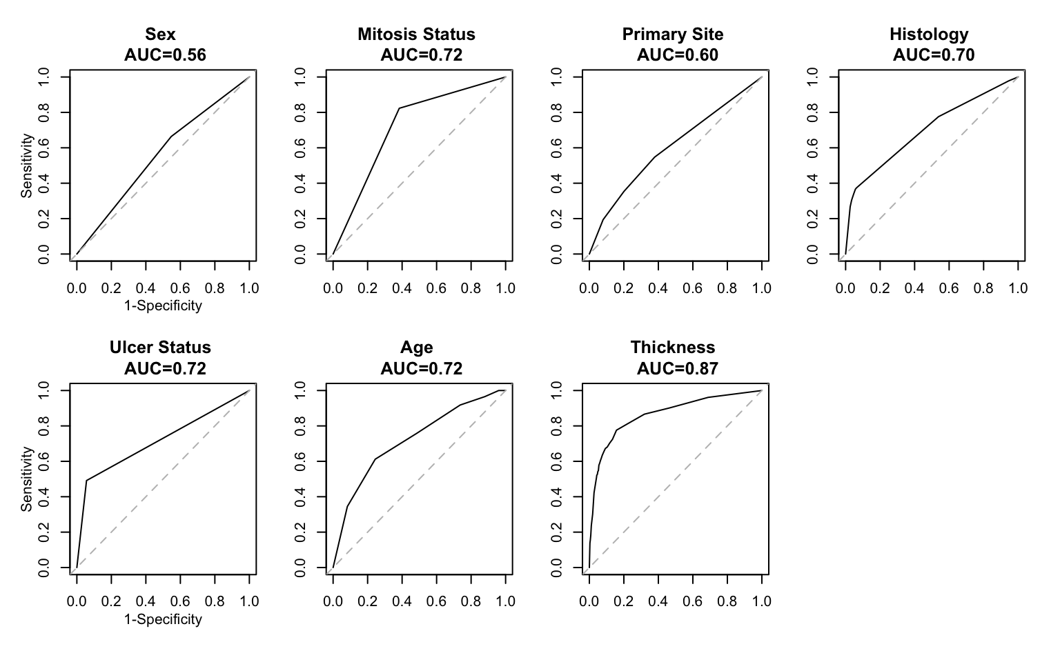
Fitting the logistic regression model allows us to construct an ROC curve and corresponding AUC for each predictor. This is important to consider separately because significant association, as seen in Table 3, will not necessarily imply high predictive ability. Given the model fits above, we can estimate each subjects probability of death as for each variable. Using this quantity as a ‘diagnostic’, we calculate the operating characteristics sensitivity and specificity for all possible values () of . Sensitivity represents the true positive fraction, and specificity the true negative fraction, and tell us for a given cut point , how well the predictor variable from the logistic regression model discriminates between those who die within 5 years and those who do not.
A plot of 1-specificity versus sensitivity for all gives rise to the ROC curve. The area under the ROC curve - the AUC - is an overall statistic, that we use to inform how well the model predicts death. A value of AUC=1 means 100% of the outcomes were correctly predicted by the fitted model. If the ROC curve follows the 45 degree line, the AUC will be close to 0.5, indicating no predictive ability of the model - effectively a coin toss. Figure 1 below shows the ROC curves for each predictor variable, along with their AUC. Thickness (of the melanoma) has the largest AUC at 0.87 indicating it best predicts death within 5 years, despite the fact that its effect size in Table 3 was not the largest. The AUC can also be interpreted as the probability that a randomly chosen subject with has a higher value than a randomly chosen subject with . The AUC resulting from the training data (here, the entire dataset) will inherently be overly ‘optimistic’, so it is important that we use a validation procedure later when comparing predictive performance between the two models.
Understanding the strength of these predictors alone, we now ask how strong they are when used in conjunction. We will consider two different prediction models: the logistic regression model again, and the naive Bayes model. The latter is considered a machine learning approach, and is more involved than the logistic regression model. One question we are interested in answering is whether our ability to estimate model tuning parameters leads to any substantial payoff in terms of our ability to predict death within 5 years.
We fit the multivariate regression model:
where represents the 5 primary sites (P1 is the referent group), and represents the 9 histologies (malignant melanoma is the referent group).
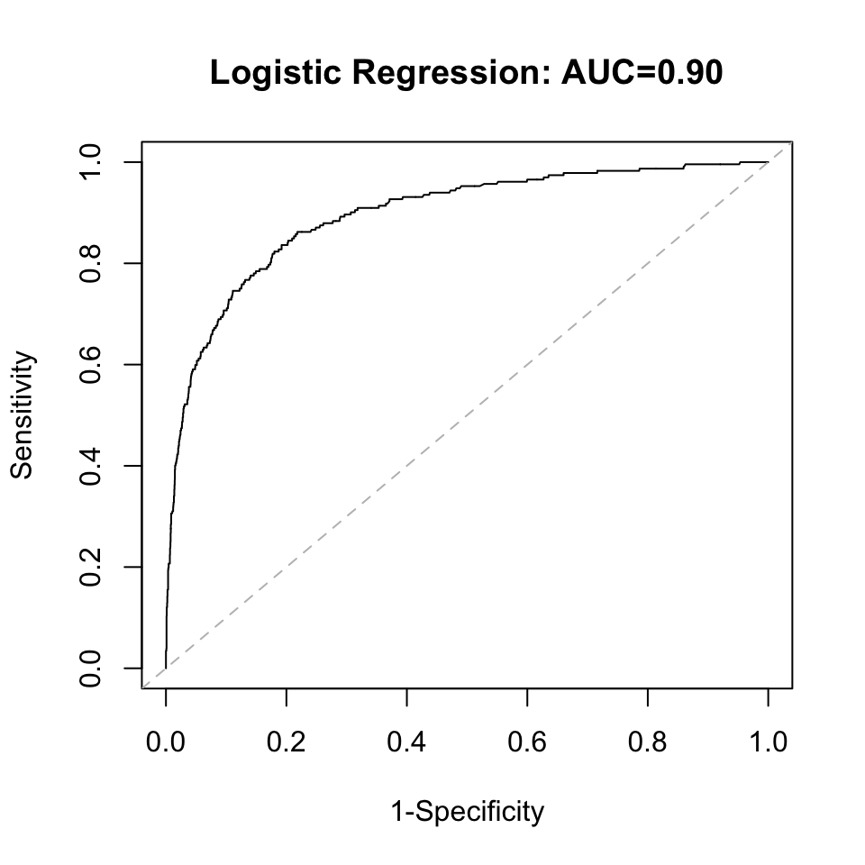
When taken together, sex is no longer significant in the model. Age, ulcer status, mitosis status, and thickness are all highly significant, while only the P2 primary site is significant relative to P1. Nodular Melanoma and Epitheliod Cell Melanoma are significant relative to the Malignant Melanoma histology. Again, significant association does not imply high predictive ability so we evaluate the predictive ability by looking at the AUC. Under the multivariate model, the AUC increased to 0.90, though this will be corrected through internal bootstrap validation. Bootstrap validation is selected instead of splitting the dataset into a training and test set because of the low event rate. The logistic regression and Naive Bayes model will be validated concurrently.
| Variable | Parameter | Odds Ratio | Wald Stat. | P-value | ||
|---|---|---|---|---|---|---|
| Intercept | 0.90 | -0.11 | 0.02 | -4.86 | <0.01 | |
| Sex (Ref.=Male) | : Female | 0.99 | -0.01 | 0.01 | -1.18 | 0.24 |
| Age (in decade) at Dx | 1.02 | 0.02 | 0.00 | 6.56 | <0.01 | |
| Ulcer Status (Ref.=Absent) | : Present | 1.17 | 0.16 | 0.02 | 10.86 | <0.01 |
| Mitosis Status (Ref.=Absent) | : Present | 1.02 | 0.02 | 0.01 | 3.04 | <0.01 |
| Thickness (mm) | 1.06 | 0.06 | 0.00 | 18.23 | <0.01 | |
| Primary Site (Ref.=P1) | : P2 | 1.05 | 0.05 | 0.02 | 3.24 | <0.01 |
| : P3 | 1.01 | 0.01 | 0.01 | 0.82 | 0.41 | |
| : P4 | 1.00 | 0.00 | 0.01 | 0.02 | 0.99 | |
| : P5 | 1.02 | 0.02 | 0.01 | 1.45 | 0.15 | |
| Histology (Ref.=Malignant Melanoma) | : Nodular Melanoma | 1.14 | 0.13 | 0.02 | 6.18 | <0.01 |
| : Amelanotic Melanoma | 0.90 | -0.10 | 0.06 | -1.62 | 0.11 | |
| : Lentigo Maligna Melanoma | 0.98 | -0.02 | 0.02 | -1.32 | 0.19 | |
| : Superficial Spreading Melanoma | 1.00 | -0.00 | 0.01 | -0.29 | 0.77 | |
| : Acral Lentiginous Melanoma | 1.08 | 0.08 | 0.04 | 1.98 | 0.05 | |
| : Desmoplastic Melanoma | 0.97 | -0.03 | 0.04 | -0.95 | 0.34 | |
| : MM in Giant Pigmented Nevus | 1.04 | 0.04 | 0.06 | 0.71 | 0.48 | |
| : Epitheliod Cell Melanoma | 1.16 | 0.15 | 0.07 | 2.21 | 0.03 | |
| : Spindle Cell Melanoma | 0.97 | -0.03 | 0.04 | -0.92 | 0.36 |
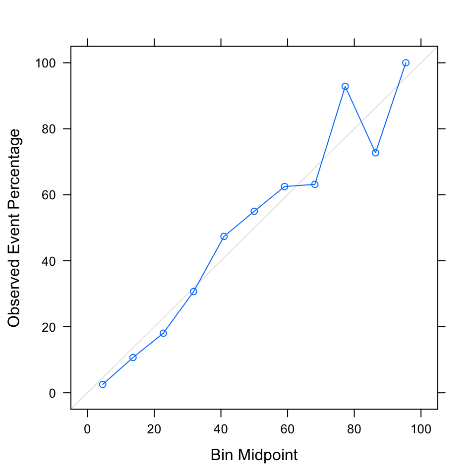
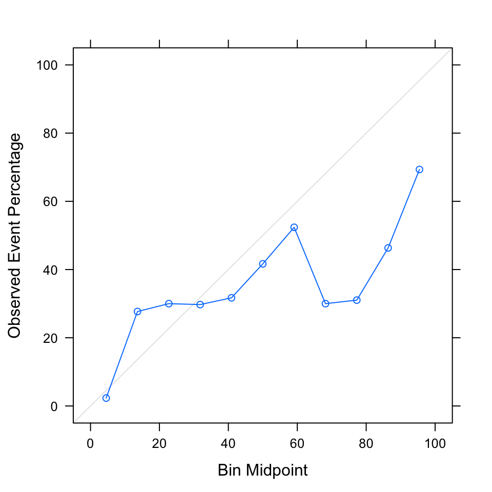
It is important to examine model calibration prior to validation, which looks at whether the model is predicting an accurate number of events for intervals of the risk score, . For example, we’d like to see that subjects with a risk score between 0 and 0.1 contribute about 12 out of 232 (0.05%) of the total number of observed events, since 0.05 is the midpoint of the risk score interval. We examine calibration using a calibration plot; a plot that follows the 45-degree line indicates good model calibration. A model that predicts well but is poorly calibrated is ultimately not useful, as it is over-predicting the outcome of interest for some individuals and under-predicting for others. The logistic regression model has good model calibration, noted by the blue line that roughly follows the 45-degree line in Figure 3. The exception is the high risk groups, where there is some over-prediction and under-prediction.
The logistic regression model is made up of a linear combination of variables, while the Naive Bayes model is represented entirely by probability statements: When is categorical, and is estimated using table proportions, and the prior class probability is also estimated from the data. For continuous , the distribution can either be estimated using a normal kernel, or a nonparametric kernel; this choice serves as the tuning parameter for the model. Additionally, we can include a tuning parameter for smoothing any marginal probabilities that are equal to 0, called the Laplace correction which adds a small value to the probabilities. We will consider values 0 (no smoothing), 0.5, 1, and 2. One limitation of this model is that in order to improve computation, we assume the covariates are independent, which is unlikely to be true. However it enables us to calculate joint probabilities as the product of marginal probabilities; studies have shown the Naive Bayes model still maintains good model performance relative to other machine learning methods under the independence assumption.
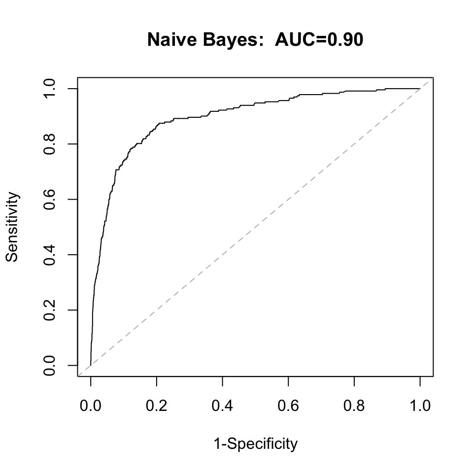
We use leave-one-out cross validation to determine the tuning parameters using the AUC as the performance metric. The model performed the same regardless of Laplace correction, so we select 0, no smoothing. Model performance was better using kernel density estimates for the covariate distributions. The AUC to evaluate the predictive ability of the Naive Bayes model is 0.90, the same as that of the logistic regression model.
Looking at the calibration plot, however, reveals that the model is poorly calibrated. There is vast overestimation for a majority of the risk intervals. Fitting the another Naive Bayes model to the original model’s predictions is a tool for recalibrating a model. Doing so overcorrected and resulted in excessive underestimation (data not shown), so we retain the original Naive Bayes model.
Now that both models have been developed, we use internal bootstrap validation to correct the model performance, since it will always be overly optimistic when using the exact data the model was built on.
| Training AUC | Validation AUC | |
|---|---|---|
| LR Model | 0.895 | 0.883 |
| NB Model | 0.895 | 0.891 |
After validation, the predictive ability of the logistic regression and naive Bayes model reduced to 0.88 and 0.89. Given the relatively small dataset, and the straightforwardness of the problem, I saw no reason a priori that the machine learning model would outperform the logistic regression model. These results confirm this, as the models perform almost equally in terms of predictive performance. The logistic regression model earns a leg up though, in having much better model calibration. It is well known that Naive Bayes models, in general, do not tend to have great model calibration.
In the absense of a sentinel lymph node biopsy and knowing whether the cancer has entered the lymphatic system, we still have a good ability to predict death within 5 years. We can infer from the univariate analysis that thickness is the variable that contributes the most to the predictive ability, which makes sense given that thicker lesions would correspond to more advanced and aggressive disease. We were able to confirm that we can maintain a high predictive ability in the absense of information from a SLNB, which is important given there are multiple subsets of patients who will not have this information. One limitation of the presented work, and a option to extend the analysis, is to look at prediction on an individual level. The AUC is a population-based metric and tells us here that we are predicting almost the right number of deaths across the study population. It does not tell us whether those predicted to die within 5 years are those who actually died within 5 years in the dataset. A confusion matrix would help to understand this aspect of the predictions.